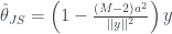
Suppose you have a sample drawn from a multivariate normal distribution in dimension . From this observation, you want to find a “good” estimate for . We will define our “good” estimate as such that expected value of the Euclidean distance between and is small. An obvious and reasonable choice would be to take . Surprisingly (at first), there are other estimators which are better. The most well-known estimator which provably dominates this estimate is the James-Stein estimator:
.
Notice this shrinks our naive estimate toward the origin. With this in mind, the surprise (somewhat) fades as the pictures below give pretty clear general intuition.
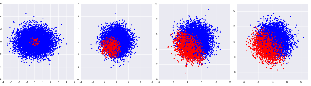
Each image is 10,000 points drawn from in projected onto a plane. Each image has a different mean; where is moving from left to right. We then shrink each point toward the origin according to the James-Stein estimator. The blue dots represents points which would improve (are closer to the true mean) if we used James-Stein as opposed to just the original data point. The red represent points which are worse. In any case more points improve as they are sucked toward the origin, and on average, the James-Stein estimate is better regardless of mean.
There are many variants of the James-Stein estimator. For example, there is nothing special about shrinking toward the origin. Also note the red points in the image on the left; for points with small norms, the multiplier in the James-Stein estimator is negative and actually pushes the estimate away from the origin. This too can be easily remedied. It seems the only magic in James-Stein concerns the amount of shrinkage applied. Where does the multiplier in the James-Stein estimator come from? We cannot shrink too much or too little. If we had some a priori idea for what should be, we could chose this as our point to shrink toward and hope to get something like the image on the left as opposed to the one on the right. This feels very Bayesian. In fact, the multiplier can be readily obtain from a Bayesian estimate of .
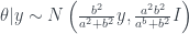
Let’s assume we don’t know , but we do know (our likelihood). We know this conditional distribution as it represents a known measurement process. We believe (our prior). We are taking this prior centered at , but the mean of the prior will dictate towards which point your estimate shrinks. For now, let’s also suppose we somehow know . Our goal is then to estimate (our posterier). This is a direct application of Bayes’ theorem which states the pdf of the posterior is proportional to pdfs of likelihood times the prior. Using this and the pdfs for normal distributions, it is not too hard to derive that
.
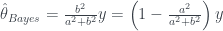
With this posterior distribution, we should take our estimate of to be
.
Indeed we have shrunk our estimate according to our prior, but this isn’t yet the James-Stein estimator. Recall we assumed we knew . What if we have some idea for what may be, but we have no clue about ? Well, we can estimate from the data ; this would fit into the category of empirical Bayes methods.
Given , if our goal is to estimate , we don’t really care about . Thus we look at the marginal distribution from which was drawn. Again, using the pdfs for our prior and likelihood, we integrate over and discover the marginal distribution so that
.
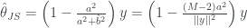
As we want to estimate , we should take
where we had to take the expected value of an inverse chi-squared distribution. Finally, we substitute our estimate for into our previous Bayes estimate , and we get the James-Stein estimate:
.
We see the James-Stein estimator is precisely the expected value of the poterior for using an empirical Bayes’ estimate. That’s great, but is it really that much better than the usual maximum likelihood estimate ? Like most things, it depends. If truly is , we can calculate
.
So if our prior is correct, the savings can be huge in high dimensions. Of course, the improvement deteriorates with worse priors, but we can calculate more generally
In the Bayes’ estimate we see the effect of a poor prior in the term, but averaging over all , this is an improvement over the max likelihood estimate. It would be nice to have , but this has proven to be a difficult term to evaluate due to the norm in the denominator. In fact, all the James-Stein related theorems I’ve found prove the James-Stein estimator dominates the max likelihood estimate for any but say nothing about the magnitude of the improvement in terms of . Still, in practice, the benefits are often significant which is why the James-Stein estimate is more than just a novelty.
As far as I can tell, the intuition that the James–Stein estimator shrinks the estimate only holds whenever $\lVert y \rVert^2 \geq (m-2)a^2$. Suppose, for instance, that $a^2 = 1$, $m = 3$, and $y = (1e-5, 1e-5, 1e-5)$. Then $\hat{\theta}_{\mathrm{JS}}(y) = -(1e4, 1e4, 1e4)$; the estimate blows up, as $y$ approaches the origin.
On the other hand, the Bayesian estimator based on $\theta \sim N(0, b^2I)$ clearly shrinks the ML estimate, so the equivalence of the two estimators will also only hold in that same regime. (Indeed, the estimate of $b^2$ becomes negative for $\lVert y \rVert^2 < (m-2)a^2$.)
Looks like you didn’t distribute. The y in the numerator will keep the JS estimate from blowing up. The example you are trying to describe is exactly what is happening with the red dots in the image on the far left. For these y’s close to the origin the JS estimate gets pushed away from the origin, but not too far. For this case where you end up “shrinking” toward the true theta (here the origin), the intuition that the estimate shrinks should be interpreted as on average.
The $y$ in the numerator is not enough to keep the estimator from pushing the estimate arbitrarily far from the origin. For the sake of example, assume that $a^2 = 1$, $m = 3$, and that $\lVert y \rVert^2 = 1/(n+1)$ for some $n > 0$. Then $\lVert \hat{\theta}_{\mathrm{JS}}(y) \rVert = \lVert (1 – (n + 1)) y \rVert = n \lVert y \rVert = n/\sqrt{n+1}$, which tends to infinity as $n \to \infty$. In particular, they certainly can get pushed away “too far” from the origin, but yes, since this happens with low probability, the expectation still improves (but again, the Bayesian interpretation fails).


 in
in  projected onto a plane. Each image has a different mean;
  where
where  is
is  moving from left to right. We then shrink each point toward the origin according to the James-Stein estimator. The blue dots represents points which would improve (are closer to the true mean) if we used James-Stein as opposed to just the original data point. The red represent points which are worse. In any case more points improve as they are sucked toward the origin, and on average, the James-Stein estimate is better regardless of mean.


![\hat{b}^2 = E\left[ \frac{||y||^2}{\chi^2_M}-a^2\right] = \frac{||y||^2}{M-2}-a^2](https://s0.wp.com/latex.php?latex=%5Chat%7Bb%7D%5E2+%3D+E%5Cleft%5B+%5Cfrac%7B%7C%7Cy%7C%7C%5E2%7D%7B%5Cchi%5E2_M%7D-a%5E2%5Cright%5D+%3D+%5Cfrac%7B%7C%7Cy%7C%7C%5E2%7D%7BM-2%7D-a%5E2&bg=ffffff&fg=333A42&s=0&c=20201002)


![E\left[||\hat{\theta}_{ML}-0||^2\right] = Ma^2](https://s0.wp.com/latex.php?latex=E%5Cleft%5B%7C%7C%5Chat%7B%5Ctheta%7D_%7BML%7D-0%7C%7C%5E2%5Cright%5D+%3D+Ma%5E2+%C2%A0&bg=ffffff&fg=333A42&s=0&c=20201002)
![E\left[||\hat{\theta}_{Bayes}-0||^2\right] = \left(\frac{b^2}{a^2+b^2}\right)^2Ma^2](https://s0.wp.com/latex.php?latex=E%5Cleft%5B%7C%7C%5Chat%7B%5Ctheta%7D_%7BBayes%7D-0%7C%7C%5E2%5Cright%5D+%3D+%5Cleft%28%5Cfrac%7Bb%5E2%7D%7Ba%5E2%2Bb%5E2%7D%5Cright%29%5E2Ma%5E2&bg=ffffff&fg=333A42&s=0&c=20201002)
![E\left[||\hat{\theta}_{JS}-0||^2\right] = 2 a^2](https://s0.wp.com/latex.php?latex=E%5Cleft%5B%7C%7C%5Chat%7B%5Ctheta%7D_%7BJS%7D-0%7C%7C%5E2%5Cright%5D+%3D+2+a%5E2&bg=ffffff&fg=333A42&s=0&c=20201002)
![E\left[||\hat{\theta}_{ML}-\theta||^2\right] = Ma^2](https://s0.wp.com/latex.php?latex=E%5Cleft%5B%7C%7C%5Chat%7B%5Ctheta%7D_%7BML%7D-%5Ctheta%7C%7C%5E2%5Cright%5D%C2%A0%3D+Ma%5E2+%C2%A0&bg=ffffff&fg=333A42&s=0&c=20201002)
![E\left[||\hat{\theta}_{Bayes}-\theta||^2\right] = \left(\frac{b^2}{a^2+b^2}\right)^2Ma^2+\left(\frac{a^2}{a^2+b^2}\right)^2||\theta ||^2](https://s0.wp.com/latex.php?latex=E%5Cleft%5B%7C%7C%5Chat%7B%5Ctheta%7D_%7BBayes%7D-%5Ctheta%7C%7C%5E2%5Cright%5D%C2%A0%3D+%5Cleft%28%5Cfrac%7Bb%5E2%7D%7Ba%5E2%2Bb%5E2%7D%5Cright%29%5E2Ma%5E2%2B%5Cleft%28%5Cfrac%7Ba%5E2%7D%7Ba%5E2%2Bb%5E2%7D%5Cright%29%5E2%7C%7C%5Ctheta+%7C%7C%5E2&bg=ffffff&fg=333A42&s=0&c=20201002)
![E\left[||\hat{\theta}_{JS}-\theta||^2\right] = \mbox{ ???}](https://s0.wp.com/latex.php?latex=E%5Cleft%5B%7C%7C%5Chat%7B%5Ctheta%7D_%7BJS%7D-%5Ctheta%7C%7C%5E2%5Cright%5D+%3D+%5Cmbox%7B+%3F%3F%3F%7D&bg=ffffff&fg=333A42&s=0&c=20201002)
![E\left[||\hat{\theta}_{JS}-\theta||^2\right]](https://s0.wp.com/latex.php?latex=E%5Cleft%5B%7C%7C%5Chat%7B%5Ctheta%7D_%7BJS%7D-%5Ctheta%7C%7C%5E2%5Cright%5D&bg=ffffff&fg=333A42&s=0&c=20201002)

As far as I can tell, the intuition that the James–Stein estimator shrinks the estimate only holds whenever $\lVert y \rVert^2 \geq (m-2)a^2$. Suppose, for instance, that $a^2 = 1$, $m = 3$, and $y = (1e-5, 1e-5, 1e-5)$. Then $\hat{\theta}_{\mathrm{JS}}(y) = -(1e4, 1e4, 1e4)$; the estimate blows up, as $y$ approaches the origin.
On the other hand, the Bayesian estimator based on $\theta \sim N(0, b^2I)$ clearly shrinks the ML estimate, so the equivalence of the two estimators will also only hold in that same regime. (Indeed, the estimate of $b^2$ becomes negative for $\lVert y \rVert^2 < (m-2)a^2$.)
LikeLike
Or, okay, $\hat{\theta}_{\mathrm{JS}}(y) = -(1e4, 1e4, 1e4) + (1e-5, 1e-5, 1e-5)$ but still.
LikeLike
Looks like you didn’t distribute. The y in the numerator will keep the JS estimate from blowing up. The example you are trying to describe is exactly what is happening with the red dots in the image on the far left. For these y’s close to the origin the JS estimate gets pushed away from the origin, but not too far. For this case where you end up “shrinking” toward the true theta (here the origin), the intuition that the estimate shrinks should be interpreted as on average.
LikeLike
The $y$ in the numerator is not enough to keep the estimator from pushing the estimate arbitrarily far from the origin. For the sake of example, assume that $a^2 = 1$, $m = 3$, and that $\lVert y \rVert^2 = 1/(n+1)$ for some $n > 0$. Then $\lVert \hat{\theta}_{\mathrm{JS}}(y) \rVert = \lVert (1 – (n + 1)) y \rVert = n \lVert y \rVert = n/\sqrt{n+1}$, which tends to infinity as $n \to \infty$. In particular, they certainly can get pushed away “too far” from the origin, but yes, since this happens with low probability, the expectation still improves (but again, the Bayesian interpretation fails).
LikeLike